
Do you know why Stradivarius violins are famous worldwide? Antonio Stradivari’s unique wood treatment and design method give them a distinctive sound that is almost impossible to copy. An episode of the BBC series “Secret Knowledge” looked at the sound of the Stradivarius, and upon analysis, it was found that its structure was slightly different from other violins.
It was noted here that the f-shaped hole of the resonator is symmetrical in most violins, but the Stradivarius violin falls slightly out of symmetry. This was the result of craftsmanship and research that focused on auditory perfection rather than visual perfection. The perfect proportions of the varnish that covers the instrument are also considered one of the reasons why the Stradivarius is so special.
In this part, we will talk about the use of NeRF (Neural Radiance Fields), one of the models that can be used for 3D modeling to help AINFT more vividly convey the unique visuals of a real Stradivarius violin. In addition, we have provided Ainize Workspace so you can train/infer the model yourself. If you want to know why you need to create an AINFT of a Stradivarius violin in the real world and bring it to the metaverse, please read the first part.
The model we will present this time is NeRF (Neural Radiance Fields). The ultimate goal of NeRF is view synthesis. NeRF receives images taken from multiple angles of an object as input. It uses these images to generate the appearance of an object from a new, non-given angle.

NeRF(Neural Radiance Fields)
Convolutional Neural Networks (CNN) structures are widely used in image processing models. However, NeRF does not use a CNN but a deep fully-connected neural network with skip connections.

The input to the model is the 3D coordinate value of each point (x, y, z) and information about the direction of the ray, i.e., information about where it is looking at (Φ, Θ). The reason for using (Φ, Θ) is that the color of each point is view-dependent. So, if a 5D coordinate value (x, y, z, Φ, Θ) is given as an input to the model, the output of the model is the (R, G, B) value of each point and the Volume Density(σ) to get the value.
Then, a 2D image is created based on the (R, G, B, σ) values by Volume rendering. The SE (squared error) per pixel between the finally obtained rendering image and the ground-truth image in the view is used as the loss. However, calculating the difference for each pixel takes a lot of efforts, so it is calculated by dividing the image into a grid and sampling only a portion of the image without comparing the entire image.
Now, when calculating the loss, instead of directly using the output of the model, how can we proceed with the result of rendering the output? Since the the volume rendering function is naturally differentiable, it is possible to find the difference between the image obtained as the output of the model and the real image.

However, it was difficult to achieve good performance using the above method alone, but additional techniques were used to obtain high-resolution results. This is where Positional Encoding becomes relevant.
Positional Encoding involves giving positional information to the input. NeRF said that positional encoding was used to better express the high-frequency part. Since the high-frequency part of an image is mainly a detailed part, Positional Encoding, can also be used to represent the detailed part of the image well. The photo on the far right of the image below is the result when Positional Encoding is not applied. You can see that the details like the Lego floor and wheels were not represented.

Using NeRF
Now let’s try to use NeRF. We couldn’t find the model presented in the NeRF paper, so we going to use NeRF_PL, an informal implementation of NeRF using pytorch-lightning. The practice environment is configured via Ainize Workspace and can be created through the link.
First, we run COLMAP with the data. COLMAP was the 3D reconstruction tool used for 3D modeling before NeRF-based models came along. We will reconstruct the camera position and pose of the object based on the image input through COLMAP. I used automatic_reconstructor for reconstruction, but a step-by-step reconstruction using COLMAP GUI would be good for performance.

The result of running COLMAP is as follows.

When the COLMAP result is obtained, we take it and convert it to the form of an LLFF data set.

A converted file in the form of an LLFF dataset has been obtained.
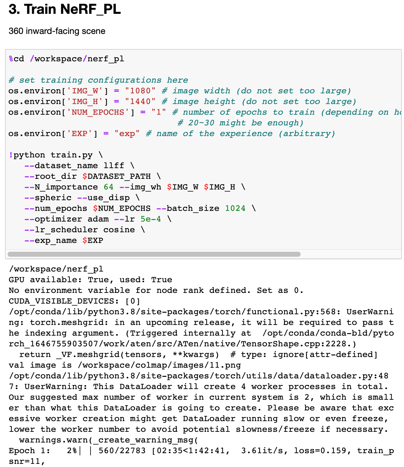
Now let’s proceed with the training. Due to time constraints, we have trained only 1 epoch.
When the training is complete, let’s run the Test.

When the test is over, a 360 rendering gif of the object is displayed.
So we looked at NeRF and even tried to use it. The NeRF we used had the disadvantage that it took too long to learn (about 5 hours per epoch). In the next part, we will learn about Instant-NGP, which improved the speed problem, and try to use it.